


This week, we looked at broadband Internet availability in countries around the world. The topic was inspired by a three-part series, "Breaking Ground," that Marketplace broadcast last week (https://www.marketplace.org/collection/breaking-ground/) about the obstacles that the United States now faces in expanding broadband access. I learned quite a bit from this series about how fiber is manufactured, and thought it might be interesting to see how the US compares with other countries.
Data and six questions
This week's data comes from the OECD's broadband statistics (https://www.oecd.org/en/topics/sub-issues/broadband-statistics.html). There are a number of different data sets that we could look at; I chose to focus on broadband penetration rates. The data set itself, in an Excel file, can be downloaded from here:
This Excel file contains two sheets, one for fixed broadband and one for mobile. We'll use both of them.
I gave you six tasks and questions to answer. As always, a link to the full Jupyter notebook that I used to perform the calculations is at the bottom of this post.
Create two data frames, one with fixed broadband info, and the other with mobile broadband info, taken from the two sheets of the Excel file. Ignore the row with overall OECD information. The country names should be the data frame's columns, and the quarters should be the rows. Combine the two data frames into a single, multi-indexed data frame.
First, let's load Pandas:
import pandas as pdNext, we'll have to load the Excel file into a single data frame. We can use read_excel to get one or more data frames back from an Excel file. If we want more than one sheet, then we can pass the sheet_name keyword argument, indicating (with a list of integers or strings) which of the sheets we want to get back. They're returned as a dict in which the sheet names (or numeric indexes) are the keys and the data frames themselves are the values. We can thus do this:
filename = '1-5-fixed-and-mobile-broadband-penetration.xls'

all_dfs = pd.read_excel(filename,
              sheet_name=[0,1]).values()
However, this code won't quite work. That's because each of the sheets contains non-data rows that mess up the reading of the data. We need to tell Pandas to ignore everything until the data starts – and more specifically, until the column names start – and then to ignore everything once the data ends.
To do this, we'll use the header keyword argument, telling it to start reading from line 3. And we'll pass nrows=38, so that we only read that many rows of data.
Next, since we want the country names to be the index, we can indicate index_col=0, to use them for the index. And finally, the .. strings should be treated as NaN values, so we pass na_values='..', adding it to the list of strings interpreted as NaN. (I didn't mention this explicitly, but it would have become obvious down the road.)
We thus end up with:
filename = '1-5-fixed-and-mobile-broadband-penetration.xls'

pd.read_excel(filename,
              sheet_name=[0,1],
              header=3,
              index_col=0,
              nrows=38,
              na_values='..').values()
This is also a good start, and returns the two data frames. However, the data frames we get here are both inverted from what we want. They have dates on the columns and country names on the rows. We'll need to transpose each of the data frames. To do that, we can use a list comprehension on the data frames we get back from dict.values, invoking transpose (or its abbreviation, T):
filename = '1-5-fixed-and-mobile-broadband-penetration.xls'

[one_sheet.T for
 one_sheet in pd.read_excel(filename,
                            sheet_name=[0,1],
                            header=3,
                            index_col=0,
                            nrows=38,
                            na_values='..').values()]
This is great, except that we now have a list of two data frames, and we actually want them to be in a single data frame. Normally, we can combine data frames with pd.concat, and we can combine them horizontally with axis='columns'. However, we want a multi-index separating the fixed from mobile values. How can we do that?
We can use the keys keyword argument, passing a list of strings that'll serve as the outer-layer names for our data frame, serving as a reminder of which original data frame each set of data came from. Here's the final query that I performed, assigning the result of pd.concat to df:
filename = '1-5-fixed-and-mobile-broadband-penetration.xls'

df = pd.concat([one_sheet.T for
                       one_sheet in pd.read_excel(filename,
                                                  sheet_name=[0,1],
                                                  header=3,
                                                  index_col=0,
                                                  nrows=38,
                                                  na_values='..').values()],
          keys=['fixed', 'mobile'],
          axis='columns')
The resulting data frame has 41 rows and 76 columns.
Turn the data frame's index (containing the quarters) into datetime values, choosing the final date of the named quarter.
First, you can tell from the fact that the question was phrased in the plural that I changed my mind while writing these questions about whether to have a single, multi-indexed data frame or two separate ones. We'll stick with the single, multi-indexed data frame in this question and in the rest of them.
The index values that we got from the Excel file were all strings of the form "Q2-2021" and "Q4-2023". In all cases, the format was Q, followed by 2 or 4, followed by a minus sign and then a year. This is fine, except that we cannot easily calculate with it. I thus decided to change these into datetime values for the final day of the second quarter (i.e., June 30th) and the final day of the fourth quarter (i.e., December 31st).
First, we need to turn the strings into something that pd.to_datetime will recognize. I chose to do that with another list comprehension, this time over all of the index values. Since each index value is a string, we can run str.replace , changing Q2- to 30-06- and Q4- to 31-12-.
If we make this transformation, and set dayfirst=True in our call to pd.to_datetime, then we'll get a datetime value. The list comprehension returns a list of datetime values, which we assign back to the index, turning our data frame into a time series:
df.index = [pd.to_datetime(one_index
                           .replace('Q2-', '30-06-')
                           .replace('Q4-', '31-12-'), dayfirst=True)
                     for one_index in df.index]
Our data frame is now what we originally wanted – the two sheets from the Excel file have been merged into a single data frame, albeit transposed from how they were presented there.
Get the mean number of fixed broadband users per country, in all of 2023. Which five countries have the greatest number per 100 people? How about mobile broadband? Is there any overlap between these two lists of countries?
Let's start by using .loc in its two-argument form to get all rows in which 2023 is the year, and where the column is fixed:
(
    df.loc['2023', 'fixed']
)
Notice that if we pass just '2023' to .loc when the index is a time series, Pandas returns all rows for which the year is 2023, treating the smaller time measurements as wildcards.
This returns two rows, one for each quarter that we got data from in 2023. We can calculate the mean across all of 2023 for each country by invoking mean on the data frame. This returns a series, one in which the data frame's columns are the index:
(
    df.loc['2023', 'fixed']
    .mean()
)
Finally, we invoke nlargest on the resulting series, getting the five countries with the largest fixed-Internet penetration in 2023:
(
    df.loc['2023', 'fixed']
    .mean()
    .nlargest(5)
)
The results:
France         46.960
Switzerland    46.550
Korea          46.405
Norway         46.045
Germany        45.425
Name: 2023-12-31 00:00:00, dtype: float64
What I found particularly amazing is that the best fixed-line broadband penetration that an OECD country had in late 2023 was still only about 46 percent.
What about mobile? We can run an almost identical query:
(
    df.loc['2023', 'mobile']
    .mean()
    .nlargest(5)
)
The result:
Japan            201.515
United States    186.560
Estonia          183.710
Finland          160.410
Israel           145.900
dtype: float64
I'm going to assume that numbers above 100 (which they all in this case) refers to people with more than one mobile device.
I asked you to find whether these lists overlap at all. With only five countries per list, we can look and decide. But what if we want to check in a more automated fashion? We can take advantage of the fact that Pandas indexes operate in some ways like sets. There's even an intersection method, which returns the common values in two indexes.
We can check by getting the index from the top-five fixed-line Internet service, and invoking intersection on the top-five mobile Internet countries. The result will tell us which places are at the top of both lists:
(
    df.loc['2023', 'fixed']
    .mean()
    .nlargest(5)
    .index
    .intersection(
        df.loc['2023', 'mobile']
        .mean()
        .nlargest(5)
        .index
    )
)
The result? No overlap at all; we get an empty object. So no countries are at the top in both.
For each country, find the year in which the mobile broadband penetration grew the greatest amount (by percentage), year over year. Plot this as a histogram, to see the number of countries with greatest growth per year.
In this question, I asked you not to find the years with the greatest mobile penetration, but rather with the greatest change in penetration for each country.
First, we need to get the mean values for each year, rather than for each half-year. To do that, we'll use resample, telling Pandas that we want to calculate the mean for all of the values in a given year (1YE):
(
    df['mobile']
    .resample('1YE').mean()
)
Now that we have the annual data, we can invoke pct_change to find how much the penetration changed from year to year:
(
    df['mobile']
    .resample('1YE').mean()
    .pct_change()
)
The result is a data frame in which the index contains years (or more accurately, the last day in each year), the columns contain country names, and each value reflects the percentage change in broadband penetration from the value just above it.
How can I find, for each country, the year with the greatest increase? The idxmax method, which returns a series whose index contains country names (i.e., the data frame's columns) and the values are the dates (from the data frame's index) with the highest value for that country.
Since we want a histogram of years, we'll retrieve the year using dt.year , taking advantage of the dt accessor for datetime values. And then finally, we can invoke plot.hist, creating a histogram from our data. The height of the bar represents the number of countries for whom that year marked the greatest boom in broadband installation.
Here's what my histogram looked like:
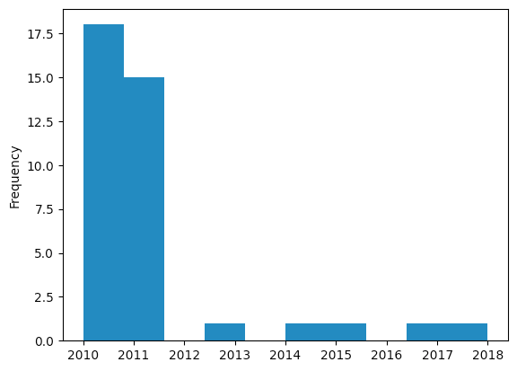
We can see that there was a huge number of countries that stepped up their investment in mobile broadband in 2010 and 2011. Ever since, a handful of countries have done so each year, but that was the biggest jump.
Are there any countries with more than 100% mobile penetration in a given quarter?
I mentioned earlier that we can see greater than 100 percent mobile penetration in a number of countries. Where does this happen?
We can find out most easily by executing this simple query:
mobile_df > 100
This returns a data frame with the same index and columns as we saw before, but with boolean values indicating whether the value was greater than 100. We can then invoke sum on the data frame, adding up all of the 1s and 0s. For each quarter in which there was >100 percent mobile penetration, the result will go up by 1.
We can then invoke sort_values to get them in order which will help us to find those that are getting more than 100% penetration, and those that never did:
(
    (df['mobile'] > 100)
    .sum()
    .sort_values()
)
And here are the results:
Italy               0
Mexico              0
Slovak Republic     0
Slovenia            0
Greece              0
Germany             0
Türkiye             0
Hungary             0
Belgium             0
Colombia            0
Canada              0
Portugal            1
Costa Rica          2
France              4
Czechia             4
Chile               6
United Kingdom      9
Spain              10
Switzerland        10
Lithuania          10
Luxembourg         10
Austria            10
Israel             11
Norway             12
Netherlands        12
Poland             12
Latvia             13
New Zealand        13
Iceland            16
United States      19
Estonia            19
Denmark            21
Japan              22
Finland            22
Australia          23
Sweden             24
Korea              25
Ireland            29
dtype: int64
We can see that a good number of countries never had even one quarter with more than 100% mobile penetration.
Have there been cases of decreases in mobile broadband? List the countries and years where this happened.
Finally, we think of mobile broadband as only increasing. I thought it would be interesting to ask if there were any cases of decreases in mobile broadband percentages.
First, we'll grab the mobile values and invoke pct_change:
(
    df['mobile']
    .pct_change()
    .stack()
    .loc[lambda s_: s_ < 0]
)
We now have a data frame in which the columns are country names, and the rows are dates. How can we find the dates and countries that were negative?
The easiest thing is to take the columns (i.e., the country names) and move them into the index, creating a series with a two-level multi-index (dates and country names). The values will be the same values as we had before, but now they'll be in a 1D data structure.
We can then use loc along with lambda to find only those negative values:
(
    df['mobile']
    .pct_change()
    .stack()
    .loc[lambda s_: s_ < 0]
)
The result contains 160 elements, of which we can see a small sample here:
2010-06-30  Greece       -0.069467
            Spain        -0.015761
2010-12-31  Israel       -0.008108
            Luxembourg   -0.019823
            Mexico       -1.000000
                            ...
2023-12-31  Norway       -0.009982
            Poland       -0.009420
            Spain        -0.000893
            Sweden       -0.029900
            Türkiye      -0.005983
Length: 160, dtype: float64
And that's about it! You can get my Jupyter notebook here: https://drive.google.com/file/d/1Lw3D723ughEtiK8RvTaw4mni9J2Y--1X/view?usp=sharing
Until then,
Reuven