


This week, we looked at the "Sahm rule," a metric created by economist Claudia Sahm (https://en.wikipedia.org/wiki/Claudia_Sahm) to determine if the government should worry enough about people's well-being to start giving them aid. Although it was created for a different purpose, the Sahm rule has come to be widely used as a tool for real-time recession detection — something that is normally only evaluated and determined after-the-fact by the National Bureau of Economic Research (NBER, https://www.nber.org/).
Over the last few weeks, I have seen numerous mentions of the Sahm rule being used to determine whether the US is currently in a recession. Things on the economic front look problematic because of Trump's tariffs, government cuts, expulsions of immigrants, large downturns in both stocks and bonds, and stubbornly high inflation. Trump is also changing his government's policies on an almost daily basis, making it difficult for businesses to plan. And more changes are in the works, with Trump's administration promising 90 bilateral trade deals within the next 90 days (https://www.nytimes.com/2025/04/23/business/economy/trump-tariffs-trade-deals.html?unlocked_article_code=1.CE8.ldm_._K_qIMnwRd89&smid=url-share). It might feel like a recession, but the NBER will only make that determination retrospectively, which makes it even harder to understand what's happening, and what should be happening.
This week, we'll look at recent US economic data to determine whether a recession has begun, at least according to the Sahm rule. Along the way, we'll get to explore some interesting Pandas functionality, including window functions, that are used in these calculations.
Data and five questions
This week, we'll be performing calculations using the Sahm rule. We'll get our data from FRED (https://fred.stlouisfed.org/), the online economics portal run by the St. Louis Federal Reserve.
Learning goals this week include working with APIs, window functions, dates and times, and plotting.
If you're a paid subscriber, then you'll be able to download the data directly from a link at the bottom of this post (although you should really use the API), download my Jupyter notebook, and click on a single link that loads the notebook and the data into a browser-based (i.e., WASM) version of Marimo. If you're wondering why I'm using Jupyter rather than Marimo, given how much I liked using it last week – it's largely a matter of inertia; I may well switch to Marimo in the near future, but I'll always make have a version in Jupyter you can download and use.
Also: A video walk-through of me answering this week's first two questions is on YouTube at https://www.youtube.com/watch?v=k6lvCpUJsRk. Check out the entire Bamboo Weekly playlist at https://www.youtube.com/playlist?list=PLbFHh-ZjYFwG34oZY24fSvFtOZT6OdIFm !
Here are my five tasks and questions for you:
Register for an API key with FRED. Install fredapi. Download the UNRATE data set from FRED. What kind of data does it return? What type of index does it have? What kind of data does it contain? When does the data set start, and when does it end? Create a line plot, showing the US unemployment rate in the data set; do any dates stand out for you?
In order to use the FRED API, you'll need to register for an API key. This is free of charge and takes very little time. First, you need to register for a FRED account, clicking on "create a new account" at https://fredaccount.stlouisfed.org/login/secure/ .
Once you have done that and signed in, then you can go to https://fredaccount.stlouisfed.org/apikey and request an API key:
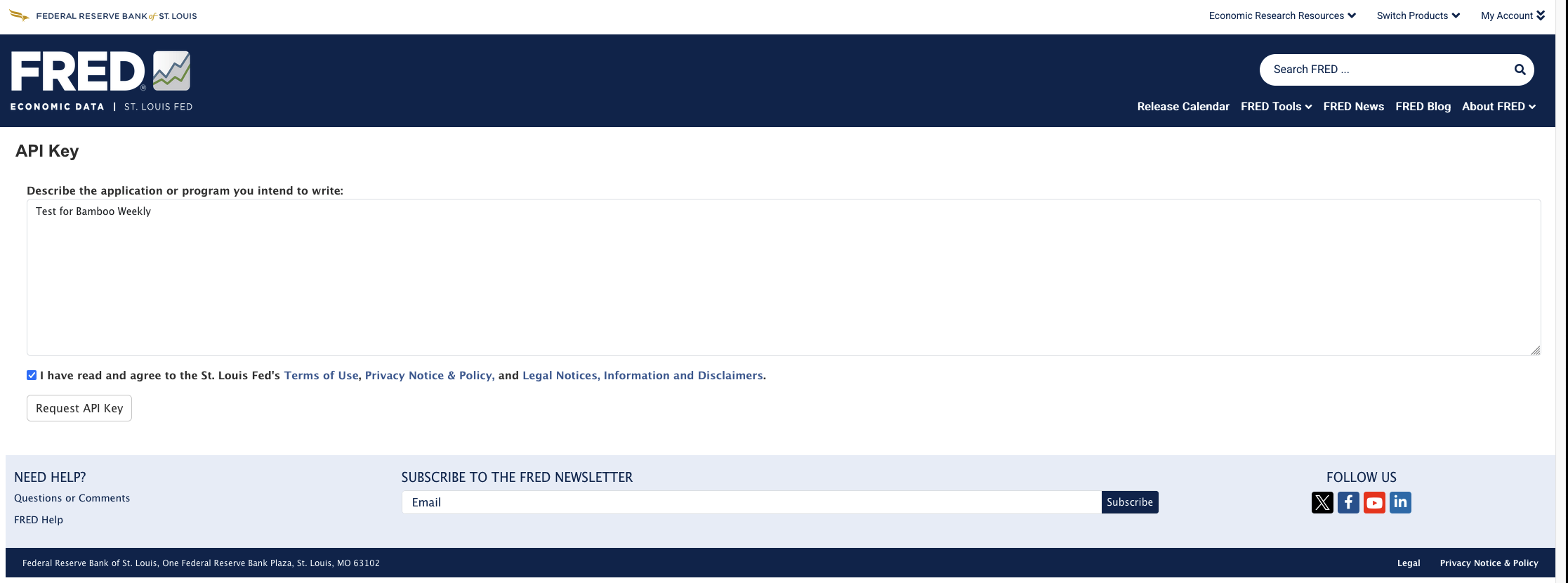
Immediately after clicking on "request key," you'll get a new key, a 32-character number in hexadecimal:
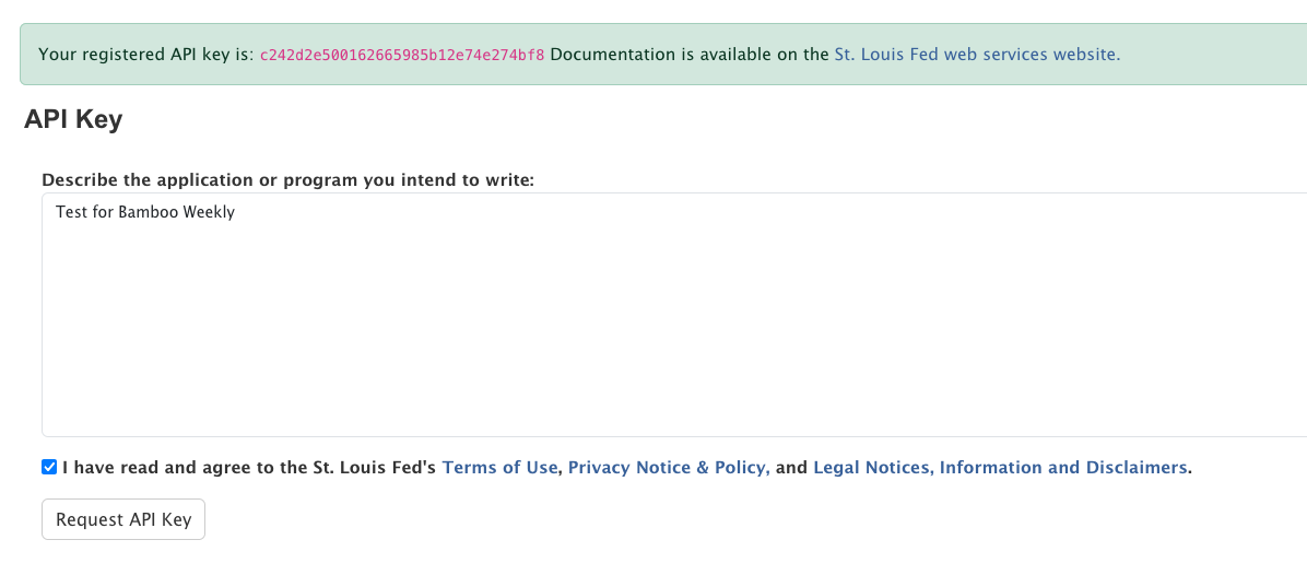
You can have multiple API keys, creating new ones and removing old ones as you deem appropriate at https://fredaccount.stlouisfed.org/apikeys . Unlike many commercial API providers, which only display API keys when you create them (to avoid security issues), FRED displays all of your keys on your key-management page. So don't feel like you have to put the key in a secure space, to avoid problems if you lose it.
With the API key in hand, we can get to work. The first thing we'll do is load up Pandas:
import pandas as pdWe're going to use the fredapi package from PyPI (https://pypi.org/project/fredapi/), which allows us to retrieve via the FRED API with little or no hassle. The package documentation says that we can retrieve a data set from FRED as follows:
from fredapi import Fred
fred = Fred(api_key='insert api key here')
data = fred.get_series('SP500')
At first, I thought that it would make sense to copy their code more-or-less verbatim, putting my FRED API key into a variable, using that variable, and then retrieving the UNRATE:
from fredapi import Fred
fred_api_key = 'c242d2e500162665985b12e74e274bf8'
fred = Fred(api_key=fred_api_key)
data = fred.get_series('UNRATE')
As I like to say in such situations, "Unfortunately, this works." That is, invoking fred.get_series works in this case. However, you should feel very, very uncomfortable with an API key hard-coded in your software. You could accidentally put it in a GitHub repository, or share it with other people – and while the FRED API is free to use, you still don't want to share your keys with other people.
For that reason, it's usually best to put your key in an environment variable, a file, or a configuration database. For example, I put my FRED key in a file in my home directory, .fred_api_key, with the single line:
c242d2e500162665985b12e74e274bf8Then, in my program, I wrote:
fred_api_key = open('/Users/reuven/.fred_api_key').read().strip()

from fredapi import Fred
fred = Fred(api_key=fred_api_key)
s = fred.get_series('UNRATE')
In other words, I used open to open the file for reading, read the entire thing into memory as a string, ran str.strip to remove any leading/trailing whitespace, and assigned the result to the same variable, fred_api_key. Even if I share my Jupyter notebook with other people, I don't have to worry that they'll be able to use my key.
(And yes, I will have deleted the key I mention by the time you read this.)
After invoking fred.get_series, I have a Pandas series. Let's examine it a bit, first using s.info:
s.info()The result:
<class 'pandas.core.series.Series'>
DatetimeIndex: 927 entries, 1948-01-01 to 2025-03-01
Series name: None
Non-Null Count  Dtype
--------------  -----
927 non-null    float64
dtypes: float64(1)
memory usage: 14.5 KB
In other words, the series has a dtype of float64, consuming 14.5 KB of memory. It contains 927 elements, indexed with datetime values, ranging from January 1st, 1948 to March 1, 2025.
A DateTimeIndex means that we can, if we want, retrieve values using .loc by specifying partial dates, or use resample to perform time-based grouping operations. It's a very convenient thing to have around, even if we won't be doing much with it in these exercises.
For example, we can create a line plot of the data:
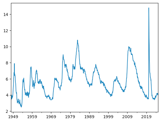
Notice that Pandas only displays the years; it's smart enough to know that printing the months (or days) would just clutter the display, given the long span of time we're displaying.
We can see a few spikes in unemployment in the last 50 years:
- Around 1980, when the Fed (led by Paul Volcker) dramatically increased interest rates to stop stagflation
- Around 1992, when there was a recession (helping Bill Clinton win the presidency)
- Around 2000, when the dot-com bubble imploded
- In 2009, when the Great Recession's effects were really felt
- In 2020, when the covid pandemic halted the world economy
Do we see an uptick in unemployment? If we look at the last part of the graph, the answer is "yes." But it doesn't seem as dramatic as the others – although you could argue that it's simply too early to tell. The Sahm rule tries to look at the most recent few months, and determine if recent unemployment contrasts enough with the previous year to warn of a recession.
Calculate, for the entire data set, the 3-month moving average for the national unemployment rate. Put the original data and this 3-month moving average into a single data frame. Don’t include a given month’s data (e.g., May 2020) when calculating its 3-month average. Instead, use the three prior months (Feb–Apr 2020).
Normally, calculating the average (mean) on a series involves invoking the mean method: The numbers are summed and divided by the length of the series, and we get an answer:
numbers = pd.Series([11, 29, 32, 48, 53, 67, 74])
numbers.mean()
The above code returns 44.857142857142854, the mean of the numbers in the series.
But I asked you to do something different, to calculate the rolling average for each date, using the previous three months of data. In other words, I wanted to get a series back, with the same index as the input series, numbers. The value in each slot would be the mean of three values. Since the first two elements would not have three predecessors, we have NaN for those items. The result of running such a calculation on numbers would be:
NaN(instead of 11)NaN(instead of 29)- 24 (the mean of 11, 29, and 32)
- 36.333333333333336 (the mean of 29, 32, and 48)
- 44.333333333333336 (the mean of 32, 48, and 53)
- 56 (the mean of 48, 53, and 67)
- 64.66666666666667 (the mean of 53, 67, and 74)
One way to think about this calculation is that we have the numbers laid out on a piece of paper, and put a second piece of paper on top of the first one. The upper piece of paper contains a small cut-out "window" that we can slide over the lower one, exposing only three numbers at a time, on which we calculate the mean.
Pandas comes with functionality like this, known as a "window function." And what we're looking to do here is a "rolling" window, calculating the mean for elements 0-1-2, then elements 1-2-3, then 2-3-4, and so forth.
We can thus say:
numbers.rolling(window=3).mean()This gives us the following result:
0          NaN
1          NaN
2    24.000000
3    36.333333
4    44.333333
5    56.000000
6    64.666667
dtype: float64
As you can see, these results are identical to what we calculated earlier. We invoke rolling to indicate that we want to perform a rolling-window calculation, and pass window=3 to indicate the size of the window that should be used. We then invoke mean to calculate the mean on the values in the window.
The Sahm rule requires that for each month, we calculate the mean unemployment rate for the three previous months. You might think that we can thus invoke
s.rolling(window=3).mean()This results in:
1948-01-01         NaN
1948-02-01         NaN
1948-03-01    3.733333
1948-04-01    3.900000
1948-05-01    3.800000
                ...
2024-11-01    4.133333
2024-12-01    4.133333
2025-01-01    4.100000
2025-02-01    4.066667
2025-03-01    4.100000
Length: 927, dtype: float64
This might seem accurate, but it has a small, subtle bug: For each month, we want the mean of the three previous months. After performing our calculation, we'll thus need to invoke shift, which shifts the series index by 1 without modifying the data. In other words, we'll want to shift it slightly, such that the data labeled March 1st will be the mean of the months December, January, and February:
s.rolling(window=3).mean().shift(1)Now we get the result:
948-01-01         NaN
1948-02-01         NaN
1948-03-01         NaN
1948-04-01    3.733333
1948-05-01    3.900000
                ...
2024-11-01    4.133333
2024-12-01    4.133333
2025-01-01    4.133333
2025-02-01    4.100000
2025-03-01    4.066667
Length: 927, dtype: float64
As you can see, we now have NaN for three elements, and the index has shifted by 1, but is otherwise the same.
I invoked pd.DataFrame to create a new data frame. I passed it a dict, such that the dict's keys are the data frames column names and its values are the rows containing values. Note that for this to work, the two series (i.e., dict values) that I pass must be the same length. But given that I'm passing s and the result of a rolling window function on s, we'll be fine:
df = pd.DataFrame({'UNRATE':s,
                   '3_month_mean': s.rolling(window=3).mean().shift(1)})
Here's the result:
           UNRATE  3_month_mean
1948-01-01     3.4           NaN
1948-02-01     3.8           NaN
1948-03-01     4.0           NaN
1948-04-01     3.9      3.733333
1948-05-01     3.5      3.900000
...            ...           ...
2024-11-01     4.2      4.133333
2024-12-01     4.1      4.133333
2025-01-01     4.0      4.133333
2025-02-01     4.1      4.100000
2025-03-01     4.2      4.066667

[927 rows x 2 columns]