BW #104: Aviation accidents (solution)

This week, in the wake of the awful crash between a passenger plane and an army helicopter in Washington, DC, we're looking at the history of aviation accidents. Commentators stressed that air travel remains extremely safe, and that these incidents are less common than they used to be. I wanted to look at the data, and see to what degree things have improved.

Data and six questions

Our data comes from the National Transportation Safety Board (NTSB, https://www.ntsb.gov/Pages/home.aspx), which investigates transportation problems. I got the data in CSV format by going to the "aviation investigation search" page (https://www.ntsb.gov/Pages/AviationQueryV2.aspx).

I decided to cast the widest possible net, and thus submitted my query without narrowing down any of the fields. That brought me to a results page; at the bottom of the page were buttons to download the data in JSON and CSV format. I chose CSV.

I have six tasks and questions for you this week. Our learning goals this week include:

• Memory optimization (https://www.bambooweekly.com/tag/memory-optimization/)
• Working with dates and times (https://www.bambooweekly.com/tag/datetime/)
• Plotting (https://www.bambooweekly.com/tag/plotting/)
• String manipulation (https://www.bambooweekly.com/tag/strings/)

If you're a paid subscriber or a subscriber to my LernerPython + data plan, you can find links to the data file and the Jupyter notebook I used to solve these problems at the bottom of this message, along with a one-click link that opens my notebook in Google Colab.

Here are my six questions:

Create a data frame from the CSV file. Make sure that EventDate is treated as a datetime value. How much memory can you save by adjusting the dtypes from the defaults?

Let's start by loading up Pandas:

import pandas as pd

Next, we can load the CSV file into a data frame:

filename = 'ntsb.csv'

df = pd.read_csv(filename)

If we just do the above, we get a data frame. But we also get a warning:

/var/folders/rr/0mnyyv811fs5vyp22gf4fxk00000gn/T/ipykernel_68606/945768307.py:6: DtypeWarning: Columns (16,17,23,27,35,36) have mixed types. Specify dtype option on import or set low_memory=False.

Remember that CSV is a text-based format. This means that when Pandas loads a CSV file into a data frame, it tries to determine whether each column should be int64, float64, or object – the last of which basically means a string type. But it doesn't load the entire file at once, which means that its determination can be different for different parts of the file. That's what the warning means: It came to different conclusions for different chunks of the file, and it might have made bad decisions.

The warning tells us that we can fix this in a two ways: We can pass low_memory=False to pd.read_csv, allowing the entire file to be read into memory in a single chunk. We can also pass the dtype keyword argument, specifying what types we want for the columns we read.

But there is a third option, one which Pandas doesn't name: We can use PyArrow to load the CSV file. While storing the actual data in PyArrow is still somewhat experimental, the CSV-loading capabilities aren't. They are often dramatically faster than the native Pandas CSV loader, and as a nice bonus, recognize and handle datetime values, too, without needing to pass the parse_dates keyword argument. Finally, PyArrow doesn't suffer from the issues that the Pandas CSV parser does with large files.

I thus decided to load the file this way:

df = pd.read_csv(filename, engine='pyarrow')

The good news is that EventDate is indeed a datetime column. The bad news is that a large number of columns contain string values. That's not bad news by itself, but the fact that many of them are repeated string values means that we're using more memory than we need.

How much more? We can calculate and display the amount of memory used by df by invoking memory_usage on our data frame. This returns a series of integers, the number of bytes used by each column in df. The index of the returned series is the same as df.columns.

However, if we simply invoke memory_usage, we won't get the true usage. That's because our strings are stored in Python's memory, not in the NumPy backend that Pandas uses. Which means that we'll find out how much memory we've allocated to NumPy, not to the strings. This can be off by quite a bit!

We thus pass deep=True to memory_usage, and then invoke sum on the resulting series:

before_memory = df.memory_usage(deep=True).sum()
print(f'{before_memory=:,}')

Notice that I print the before_memory value inside of an f-string, with , as the format specifier after the : character. Having a comma there tells Python to put commas before every three digits. The = just before the : means that I want to print the variable name and also its value, which I've found invaluable in debugging.

On my computer, I found that the data frame consumed about 249 MB.

My question was: Can we shrink this at all?

One of the biggest wins in Pandas memory management is to use categories. If you have a string (object) column with values that repeat themselves, then switching to a category dtype can save you lots of memory. Basically, a category looks, feels, and acts the same as a string – but behind the scenes, it actually contains an integer, referring to the original string value in an array.

Rather than analyze each column separately, I decided to just convert every object column into a category dtype. To do this, I had to select all of the object columns. Thankfully, Pandas has a method that does just this, select_dtypes. I can get the names of the object columns by invoking select_dtypes('object'). Then on each column I want to switch from containing strings to categories, I can invoke astype, passing the argument 'category'.

Here's how I did that:

for one_column in df.select_dtypes('object').columns:
    print(f'\t{one_column}')
    df[one_column] = df[one_column].astype('category')

However, there was one more set of columns that I decided to shrink: The three columns that count injuries and fatalities were defined as int64, when they never went higher than a few hundred. I decided to change those columns to uint16, meaning unsigned 16-bit integers. (And yes, we could have made some of them uint8, but I decided it wasn't that big of a deal.)

How can I choose the columns I want? I decided to invoke df.filter, which lets us select columns from a data frame via a regular expression. I asked for .*Count$, meaning that I wanted the column name to end with the string 'Count'. Here's the code I used:

for one_column in df.filter(regex='.*Count$', axis='columns'):
    df[one_column] = df[one_column].astype('uint16')

Finally, I measured the memory after the optimizations, printing that memory and also how much smaller the final memory was:

after_memory = df.memory_usage(deep=True).sum()
print(f'{after_memory=:,}')

print(f'{after_memory / before_memory=:0.2f}')

The result:

after_memory=87,525,949
after_memory / before_memory=0.35

In other words: With a handful of lines of code, we managed to cut our memory usage down to 35 percent of its original size (about 87 MB), without reducing functionality.

The data frame contains 176,884 rows and 38 columns.

Display a bar graph showing, for each 5-year period in our data set, the number of flights in the United States with fatalities. Do we see a trend?

I have long heard that the number of fatal crashes in the United States has dropped considerably over the years. With this data, we can find out if that's true. First, while the data set is mostly from the United States, a number of rows describe non-US incidents. We'll first use loc and lambda to keep only those rows from the US:

(
    df
    .loc[lambda df_: df_['Country'] == 'United States']
)

Next, we only want those incidents in which there was at least one fatality. This means checking the FatalInjuryCount:

(
    df
    .loc[lambda df_: df_['Country'] == 'United States']
    .loc[lambda df_: df_['FatalInjuryCount'] > 0]
)

I asked you to look at every 5-year period in the data set. That'll require more than a simple groupby; that would work on each year, or even each month. We'll need to use resample, which only works on a time series – that is, when the index is a datetime. So we'll use set_index to move EventDate to the index, and then run resample with a period of 5YE (i.e., end of every 5 years).

But wait, what do we want to calculate for every 5-year period? I asked you to find the number of flights with fatalities. That means counting the rows, which in turn means that we can choose any column and invoke count on it. I chose NtsbNo, the ID number for the NTSB investigation:

(
    df
    .loc[lambda df_: df_['Country'] == 'United States']
    .loc[lambda df_: df_['FatalInjuryCount'] > 0]
    .set_index('EventDate')
    .resample('5YE')['NtsbNo'].count()
)

With that in place, we can now invoke plot.bar to create a bar plot. The x axis will reflect the dates in the series that resample returns, and the y axis will represent the values:

(
    df
    .loc[lambda df_: df_['Country'] == 'United States']
    .loc[lambda df_: df_['FatalInjuryCount'] > 0]
    .set_index('EventDate')
    .resample('5YE')['NtsbNo'].count()
    .plot.bar()
)

Here's what I got:

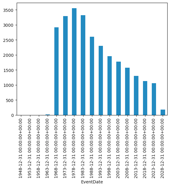
The final bar is much shorter than the previous ones because it only reflects incidents through the end of 2024, only 20 percent of the other periods. But we otherwise do we a pretty clear downward trend, from a high of 3,500 flights with fatalities in the 1970s to 1,000 in the last decade.

The NTSB data set includes information about whether the flights were amateur or commercial, and it would certainly be interesting to find how many of the problematic flights were amateur, given how many commentators mentioned that the DC flight was the first fatality of a commercial airliner in more than a decade.