BW #103: CDC data (solution)

Donald Trump has returned to the White House. This time, he wants to be sure that no government agency contradicts him. As such, he has blocked the various federal health agencies, including the Centers for Disease Control and Prevention, from communicating with their colleagues and the public until further notice. Sadly, the diseases themselves weren't cc'ed on this memo, which means that they'll continue to infect people and cause trouble, even if doctors, hospitals, and researchers aren't updated.

I decided to examine data from one affected government agency, to see the depth and breadth of what US government agencies provide. I opened the portal for publicly available data at the Centers for Disease Control and Prevention (CDC, at https://data.cdc.gov/), and clicked on the first link, leading to the National Center for Health Statistics (https://data.cdc.gov/browse?category=NCHS&sortBy=last_modified). I chose the most recent data set, "Provisional Percent of Deaths for COVID-19, Influenza, and RSV by Select Characteristics."

One set of reports from one agency doesn't do justice to what the US government's many employees do for the US and the world; for that, I would suggest reading "The Fifth Risk," by Michael Lewis (https://en.wikipedia.org/wiki/The_Fifth_Risk).

Data and six questions

This week's data set is a CSV file describing the number of deaths from each of three diseases (covid-19, influenza, and RSV) over the last few years, with week-by-week numbers separated out by ethnic group, age, and sex. You can download the file from the NCHS portal at:

https://data.cdc.gov/NCHS/Provisional-Percent-of-Deaths-for-COVID-19-Influen/53g5-jf7x/about_data

Click on the "export" button at the top of the screen, and ask to receive the download in CSV format.

This week's learning goals include:

• Multi-indexes (https://www.bambooweekly.com/tag/multi-index/)
• Working with dates and times (https://www.bambooweekly.com/tag/datetime/)
• Pivot tables (https://www.bambooweekly.com/tag/pivot-table/)
• Plotting (https://www.bambooweekly.com/tag/plotting/)
• Window functions (https://www.bambooweekly.com/tag/window-functions/)

I've enclosed my Jupyter notebook at the end of this message in two formats: (1) Downloadable, for use on your own computer, and (2) with a clickable link that opens the notebook and data set in Google Colab.

Here are my solutions and explanations:

Load the CDC's data from a CSV file into a data frame. Keep only the columns 'demographic_type', 'weekending_date', 'pathogen', 'demographic_values', 'deaths', and 'total_deaths'. Create a three-part multi-index with demographic_type, weekending_date, and pathogen. Remove rows in which the value of "pathogen" is "Combined". The "weekending_date" column should be treated as a datetime value.

Before doing anything else, I loaded Pandas:

import pandas as pd

Next, I wanted to load the data into a data frame. The easiest way to do this is with read_csv:

filename = 'cdc.csv'

df = (
    pd
    .read_csv(filename)
)

However, I asked you to do a few more things with this data. First, we want to turn weekending_date into a datetime column. We can do that by passing the column name with the parse_dates keyword argument. I also specified which columns we want to keep:

filename = 'cdc.csv'

df = (
    pd
    .read_csv(filename, 
              parse_dates=['weekending_date'],
                usecols=['demographic_type', 'weekending_date', 'pathogen',
                         'demographic_values', 'deaths', 'total_deaths'])
)

This seems fine, but aren't we missing something? I asked for us to have a three-part multi-index, which we could have set via the index_col keyword argument. However, that would have made it a bit more difficult to remove the rows in which pathogen wasn't the 'Combined' value.

I thus decided to read the data frame in without specify an index. Then I used loc and lambda to keep the non-"combined" rows:

filename = 'cdc.csv'

df = (
    pd
    .read_csv(filename, 
              parse_dates=['weekending_date'],
                usecols=['demographic_type', 'weekending_date', 'pathogen',
                         'demographic_values', 'deaths', 'total_deaths'])
    .loc[lambda df_: df_['pathogen'] != 'Combined']
)

Finally, I invoked set_index to set the index. By passing a list, I was able to create a multi-index:

filename = 'cdc.csv'

df = (
    pd
    .read_csv(filename, 
              parse_dates=['weekending_date'],
                usecols=['demographic_type', 'weekending_date', 'pathogen',
                         'demographic_values', 'deaths', 'total_deaths'])
    .loc[lambda df_: df_['pathogen'] != 'Combined']
    .set_index(['demographic_type', 'weekending_date', 'pathogen'])
)

The result is a data frame with 13,212 rows and 3 columns. Note that invoking df.shape never includes the columns used in the index.

Create a bar plot showing, for each quarter, the number of people who died in the US from influenza. Each bar should be subdivided into subplots for age group. Does any part of this data seem unusual? What might explain it?

For starters, we're only interested in those rows where the demographic_type is 'Age Group' and where pathogen is 'Influenza'. Both of those columns are part of our index, but they're in the first and third columns of the index, making it a bit tricky to retrieve matching rows using just .loc.

However, we can use .xs, the "cross-section" method we can use to retrieve selected rows from a multi-index. Since I have two values that I want to match, I'll pass a 2-element tuple, ('Age Group', 'Influenza'). I'll indicate that I want to match two levels, and which levels those are, by passing a list of the multi-index's column names:

(
    df
    .xs(('Age Group', 'Influenza'), 
        level=['demographic_type', 'pathogen'])
)

The result is a subset of my original data frame, one with only the rows and columns I want.

From this, I need to create a different data frame, one in which the rows represent each quarter (i.e., 3-month period) and the columns represent the different age groups. To do that, I'll use pivot_table, using weekending_date for the rows and demographic_values for the columns. Remember that the index and columns arguments to pivot_table get the names of categorical columns; we'll get one row/column for each unique value in each of those categorical columns.

Since we want the number of deaths for each age group at each date, I asked to use deaths as the value column and then sum as an aggregation function – although I'm pretty sure that I didn't need to specify anything, since there will be only one value for each date/age-group intersection:

(
    df
    .xs(('Age Group', 'Influenza'), 
        level=['demographic_type', 'pathogen'])
    .pivot_table(index='weekending_date',
                 columns='demographic_values',
                 values='deaths',
                 aggfunc='sum')
)

I could produce this as a bar chart, but that would create a huge number of bars, one for each week in our data set. I asked you to produce only one bar per quarter. This means using resample, a form of grouping that works on time series, i.e., data frames with datetime values in the index.

Here, we'll invoke resample with an argument of '1QE', meaning that we want to get a result for the end of each quarter, summing all of the values that fell into that quarter:

(
    df
    .xs(('Age Group', 'Influenza'), 
        level=['demographic_type', 'pathogen'])
    .pivot_table(index='weekending_date',
                 columns='demographic_values',
                 values='deaths',
                 aggfunc='sum')
    .resample('1QE').sum()

)

Finally, we can create our bar plot with plot.bar. But rather than have separate bars for each age group, I asked to stack them on top of one another with stacked=True:

(
    df
    .xs(('Age Group', 'Influenza'), 
        level=['demographic_type', 'pathogen'])
    .pivot_table(index='weekending_date',
                 columns='demographic_values',
                 values='deaths',
                 aggfunc='sum')
    .resample('1QE').sum()
    .plot.bar(stacked=True)

)

The result:

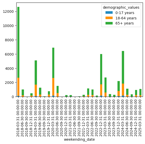
See the huge dip in influenza deaths in the center of the graph? That matches the covid-19 pandemic pretty well; since we were all at home, the virus didn't really have anywhere to go and infect others, even during the winter flu season. (We can see the seasonality of flu infections in these graphs, too.)

We also see, not surprisingly, that people 65 and older are the overwhelming bulk of flu deaths each year, and people 0-17 are a very small proportion.